EG31 MATHCAD NOTES

SESSION 1

WHAT CAN BE DONE WITH MATHCAD?

1. Combine the functionality of a spreadsheet with the WYSIWYG text and features of a word processor to generate a textbook-like document.

2. Update the entire document by making a change on any page.

3. Read data from a file and do mathematical operations such as adding a column of numbers , evaluating integrals or derivatives and invert matrices.

GETTING AQUAINTED WITH THE MENUS AND TOOLS

1. Across the top of the Mathcad window are the pulldown menus:

F ile Edit V iew Insert Format M ath Symbolics W indow H elp

2. The second line contains the standard tool icons found in a word processor along with some additional ones for Mathcad. The function of each of these icons can be identified by placing the cursor on it, without clicking, and reading the prompt that appears

3. The Math tool palette consists of eight icons. These functions can also be identified by placing the cursor on the icon. Clicking once on any of these icons makes the related function window appear.

4. The formatting toolbar, common to Microsoft Word and Excel appears just above the main Mathcad window.

To conserve screen space, any or all of the toolbars can be hidden or shown. To do this, click on the V iew menu and click on the T oolbars selection with the cursor. This will expose a menu with the choices: S tandard, Formatting and M ath. Clicking on one of these causes a check mark to either appear or disappear next to it and the corresponding toolbar to do likewise.

UNITS & PHYSICAL CONSTANTS

US CGS

feet (ft) centimeter (cm)

gram (gm) pound (lb)

second (sec) second (sec)

coulomb (coul) coulomb (coul)

Kelvin (K) Kelvin (K)

SI

meters (m) meters (m)

kilogram (kg) kilogram (kg)

second (sec) second (sec)

amp (A) coulomb (coul)

Kelvin (K) Kelvin (K)

candela (cd)

mole (mole)

Mathcad starts in SI units, unless the user specify some other system of units.

To change the units:

1. Choose O ptions from the Math pull down menu at the top of the Mathcad window.

2. Select the Units System tab at the top of the Math Options window.

3. Click on whatever default system of units that you would like to use.

4. Click on the OK button at the bottom of the window to set the new units or click on the cancel button to keep the same ones.If you set the units system to None, you can define your own units in terms of the special built-in constants 1L, 1M, 1T, 1Q, 1K, 1C and 1S which represent the dimensions length, mass, time charge or current, absolute temperature, luminosity and substance.

To display the units in the Mathcad worksheet:

1. Choose O ptions from the Math pull down menu at the top of the Mathcad window.

2. Click on the Dimensions tab at the top of the Math Options window

3. Click on the box next to Display dimensions.

4. Click on the OK button at the bottom of the window to confirm the Display dimensions mode or click on the cancel button to keep the dimensions undisplayed on the Mathcad worksheet.

A Simple Calculation

1. Click anywhere in the worksheet. You see a small crosshair. Anything you type appears at the crosshair.

2. Type 15 - 8 / 104.4 = . When you press the equals sign, Mathcad computes and

shows the results.

As you type the equation, Mathcad shows a small rectangular box called the placeholder . This holds spaces open for numbers or expressions not yet typed. As soon as you type a number, it replaces the placeholder in the equation.

3. Once an equation is on the screen, you can edit it by clicking on the appropriate spot and typing new letter, digits or operators.

4. You can type many operators and Greek letters by clicking on the Greek letters in the Math toolbar to make the Greek letter palette appear. Then simply click on the Greek letter you wish to appear at the placeholder in your equation.

Defining Variables

To clear any previous equation and define a variable t , follow these steps:

1. Click in the equation you just typed and press [Space] until the entire expression is held between the two editing lines.

2. Chose Cut for the E dit menu.

3. To begin defining t , type t: (the letter t followed by a colon). Mathcad shows the colon as the definition symbol :=

4. Type 10 in the empty placeholder to complete the definition for t .

If you make a mistake, click on the equation and press [Space] until the entire expression is between the two editing limes, as you did earlier. Then delete it by choosing Cu t from the Edit menu.

To enter another definition:

1. Press the Enter key. This moves the crosshair below the first equation.

2. To define acc as -9.8, type acc : -9.8 . Then press the Enter key again.

Calculating Results

Now that the variables t and acc are defined, they can be used in other expressions.

1. Use the mouse to place the cursor a few line below the two definitions and click.

2. Type acc / 2[Space] * t ^ 2 . the caret symbol ( ^ ) represents raising to a power. The asterisk ( * ) is multiplication and the slash ( / ) represents division. Placing the space after the 2 lets Mathcad know that the *t does not belong in the denominator but is to multiple the complete previous expression.

3. Press the equal sign key ( = ).

This equation calculates the distance traveled by a falling body in time t with acceleration acc. We had previously defined t = 10 seconds and acc = -9.8 meters per second squared.

Entering Text

To enter text, you click in an empty space and do one of the following: choose Text Region from the Insert menu or press the double-quote key ( " ).

Now do the following:

1. Click in the blank space to the right of the equations you entered. You will see a small crosshair.

2. Press " to tell Mathcad that you're about to enter some text. The crosshair is changed into a vertical line called the insertion point . the characters that you type appear behind this line. A box surrounds the insertion point, indicating that you are now in a text region. This box is called the text box. It grows as you enter text.

3. Type the words: Equations of motion.

Equations of motion

4. To enter a second line of text, press the enter key and continue to type:

for falling body under gravity.

Equations of motion

for falling body under gravity

5. To move out of the text box, click on a different spot on the worksheet or press

[Shift][Enter ].

6. To edit the text after leaving the text box, simply click on the text to reactive the text box.

Iterative Calculations

Mathcad can do repeated or iterative calculations as easily as individual ones. It uses a special variable called a range variable to perform iterations.

Range variables take on a range of values, such as the integers form 0 to 10. Whenever a range variable appears in a Mathcad equation, Mathcad calculates the equation once for each value of the range variable.

To compute equations for a range of values, first create a range variable . In this case, we will compute the results for a range of values of t from 10 to 20 in steps of 1.

1. change t into a range variable by editing its definition. Click on the 10 in the equation t : = 10. The insertion point should be next to the 10.

2. Type , 11. This tells Mathcad that the next number in the range will be 11.

3. Type ;20 . This tells Mathcad that the last number in the range will be 20 . Mathcad shows the semicolon as a pair of dots. Clicking outside the equation for t causes Mathcad to compute with t defined as a range variable. Since t takes on eleven different values, there must be eleven different answers. These are displayed in the table .

Mathcad displays on the first 16 rows of the table of calculated

values. Single-clicking on the table displays horizontal and

vertical scroll bars which can be used to view any group of 16

rows of the calculated values.

Defining a Function

Additional flexibility can be gained by defining functions. Here is how to add a function to your worksheet:

1. First, delete the table. To do so, click anywhere in the table and press the [Space] bar until everything is enclosed between the two editing lines.

2. Define the function d(t) by typing d( t ) :

and the expression : 1600 + acc / 2 [Space] * t ^ 2

The definition just typed defines a function with the name d with the argument t .

This function can be used to evaluate the expression for different values of t.

To evaluate the function at the value 3.5, type d ( 3.5 ) =.

Mathcad returns the correct value as shown below.

To evaluate the function once for each value of t defined earlier, click below the equation

and type d ( t )=.

Mathcad shows a table of values. The first two values are in exponential

(powers of 10) notation.

Formatting a Result

The display format can be set for any number that Mathcad calculates and displays. The previous table can be changed so that none of the numbers are displayed in exponential notation.

1. Click on the table with the mouse and choose Number from the Format menu. The Format Number dialog box is displayed. The number of decimal places, the use of exponential notation and whether the number is shown in decimal, octal, or hexadecimal can be selected as settings. The option button beside "Set for current region only:" should be filled in. The Format Number dialog box can also be displayed by double-clicking on the table.

2. The default setting for Exponential Threshold is 3. This means that only numbers greater or equal to 103 are displayed in exponential notation. Click to the right of the 3 , press [BkSp] and type 6 . Then click the "OK" button. The table changes to reflect the new format and 1110 is no longer shown in exponential notation.

Graphs

Mathcad can show both two-dimensional Cartesian and polar graphs, contour plots, surface plots and a variety of other two dimensional plots. These are all done in a plot region.

To create a graph

1. Click in a blank space where you would like to locate the graph and type the expression for the dependent expression which is to appear on the y-axis of your plot. Type d ( t ) and be sure that the editing lines remained displayed on the expression.

2. Choose Graph=>X-Y Plot form the Insert menu. This will produce an empty graph with placeholders on the x-axis and y-axis for the expressions to be graphed.

3. Type in t at the placeholder on the x-axis of the graph. Click anywhere outside the graph and Mathcad calculates and graphs the points as shown below.

Equation of motion for falling

body under gravity

Resizing a graph

1. Click the mouse just outside the graphics region to anchor one corner of the selection rectangle.

2. Press and hold down the mouse button and drag the mouse toward the plot region. A dashed selection rectangle emerges from the anchor point.

3. With the selection rectangle just enclosing the graphics region, let go of the mouse button. The dashed rectangle will turn into a solid rectangle with handles.

4. Move the mouse pointer to any of the handles. When it is properly positioned, it will turn into a double-headed arrow.

5. Press down and hold the mouse button and move the mouse to stretch the graphics region in that direction.

6. Once the graphics region is the right size, let go of the mouse button.

7. This operation can be repeated with any of the handles.

8. When the graph has been stretched to the desired size, click outside of the graphics region to deselect it.

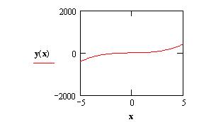
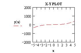
Zooming in on a portion of a graph

Sometimes it is desireable to be able to zoom in on a portion of a graph in order to find out details such as the value(s) at the intersection of two plotted equations. These types of points are of interest since they are the set(s) of values that are the solution to both equations.

Zooming Method 1:

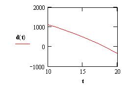
1. Click on the graph so that it appears in the solid boarder with handles. It also has numerical values at the extremes of each of its axes in addition to the usual values along each of the axes.

2. Click on the leftmost value for the horizontal axis. A cursor appears in that location.

3. Press the Delete key to remove the present value of 10 and replace it with a placekeeper.

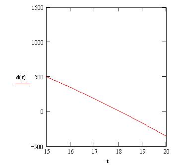
4. Type in 15 and press the Enter key. The leftmost value on the horizontal scale is changed from the default value of 10 to 15. The graph has now zoomed in on the portion of the data between the values of 15 and 20.

Note: The same steps are used to zoom out on a graph. However, the graph will only plot the values which are defined by the original range variable and the resulting values computed for the dependent variable. It will not extrapolate the plot to the new range.

Zooming Method 2:

1. Click on the graph to select it.

2. In the Format menu at the top of the window, choose G raph and then Zoom .

This causes the X-Y dialog box to appear.

3. If needed, the dialog box can be repositioned, using the mouse, to allow the complete graph to be seen.

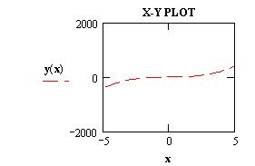
4. Within the graph region, place the mouse at a location which locates one corner of a box that you want to draw to describe the region you want to magnify.

5. Press and hold the mouse button down as you define the box around the area to be magnified by dragging the mouse through a diagonal path to describe the region to be magnified. A dashed rectangle appears as you drag the mouse to indicate the region.

6. If necessary, the region can be repositioned by positioning the cursor in the dashed box, pressing and hold the mouse button and move the mouse to reposition the dashed rectangle.

Note that the coordinates of the corners of the dashed box are displayed in the X-TY Zoom dialog box and that they change as dashed box is moved.

7. Clicking on the Zoom button redraws the graph within the dahed box as the full graph.

8. The limits of the axes are those of the dashed box. However, they can be changed as described in Zooming Method 1, above.

To unzoom a graph that has already been zoomed but which the axis limits have not been changed.

1. Click on the graph to activate its graph region.

2. Choose G raph => Zoom from the F ormat menu to bring up the X-Y Zoom box.

3. Click on the U nzoom button to get back to the previous level of zoom or click on the Full View button to see the original graph prior to any zooming.

Graph coordinates

To see a readout of the graph coordinates that make up a trace:

1. Click on the graph region to select it.

2. Choose G raph => Trace from the F ormat menu, or clic on the Trace button on the Graph Palette, to show the X-Y Trace dialog box. Reposition the box so that the entire graph can be seen, if necessary. Note that the Track Data Points box is checked.

3. In the graph region, click and drag the mouse along the trace whose coordinates you want to see. A dotted crosshair jumps from one point to the next as you move along the trace.

4. If the mouse button is released, the left and right arrrows can be used to move to the previous or next data points. The up and down arrows move to other traces on the same graph.

5. As the pointer reaches each point on the trace, Mathcad displays the x and y values of that point in the X-Value and Y-Value boxes.

6. The coordinate values of the last selected point remain in the boxes. The crosshair remains until you click outside the graph.

To copy a coordinate to the clipboard:

1. Click "Copy X "or "Copy Y". The value can then be pasted into a math region or a text region on the Mathcad worksheet, into a spreadsheet, or into any other application that allows pasting from the clipboard.

2. Click outside the graph or on the "Close" button to make the crosshairs disappear.

Formatting a graph

A graph is produced with default characteristics: numbered linear axes, no grid lines and points connected with solid lines. These characteristics can be changed for formatting the graph.

To do this:

1. Double-click on the graph to bring up the appropriate dialog box. This box contains settings for all available plot format options.

2. Click on the Traces tab in the dialog box to see the correct page.

3. Click on "trace 1" in the scrolling list under "Legend Label". Mathcad places the current settings for trace 1 in the boxes under the corresponding columns of the scrolling list.

4, Click on the arrow under the "Type" column to see a drop-down list of trace types.

5. Choose "bar" from this drop-down list by clicking on it.

6. Click on the "OK" button to show the result of changing the setting. Mathcad shows the graph as a bar chart instead of connecting the points with lines.

7. Click outside the graph to deselect it.

Building Expressions

Mathematical expressions can be created in Mathcad by simply typing in a stream of characters. Characters like * and + represent operators.

Mathcad behaves a lot like a standard word processor. As you type, characters appear behind a vertical editing line. There are, two important differences:

1. As the editing line moves to the right, it leaves behind a horizontal editing line.

2. Unless you have clicked on an equation that already has an operator in it, pressing the [Space] bar will turn the the math region into a text region. You cannot turn a text region back into a math region.

Typing in operators

Operators like the symbols + and - link variables and numbers to form expressions. These expressions are called operands . The key to working with operators is learning to specify which variable or expression is to become the operand. This can be done in two ways:

1. You can type the operator first and fill in the placeholders with operands.

2. You can learn how to use the editing lines to specify what variables or expression you want to turn into an operand.

Try creating the expression a x+y using the first method:

1. Press ^ to create the exponent operator. It appears with two placeholders.

2. Click in the lower placeholder and type the letter a.

3. Click in the upper placeholder and type + .

4. Click in the remaining placeholders and type x and y .

Now try creating the same expression using the editing lines.

1. Type a . The line beneath the a indicates the a will be the first operand of whatever operator you type.

2. Press ^ to create the exponent operator. The editing lines now surround the new placeholder.

3. Type x + y in this placeholder to complete the expression.

Now type the expression a x + y instead of a x+y .

1. Type a^x .

2. Press the [Space] bar to cause the editing line to hold the entire expression.

3. Now type + . Whatever was held between the editing lines has now become the first operand of the plus sign.

4. In the remaining placeholder, type y .

EG 31 MATHCAD EXERCISES

SESSIONS 1

Exercise 1 : Units Conversion

1. Go to options in the Math pull down menu. Select the Dimensions tab and click on the box next to "Display dimensions".

2. In the box next to "Mass" type kg . In the box next to " L ength" type m . In the box next to "Time" type sec .

3. Type in the following:

4. Now type F = to get the answer with units:

To change the units:

Click on the placeholder to the right of the units and type in dyne and press the Enter key.

Exercise 2: X-Y plots

1. Define the range of the variable x to start at -8 and end at +8 and to increment by 0.1

2. Define the equation for the dependent variable y(x) as 3x3 + 7x +3

3. Plot the graph.

4. Redefine the range of the variable x to start at -5 and end at +5 .

5. Add the title X-Y PLOT (Hint: double click on the graph)

6. Deselect Autoscale

7. Change the plotted line to a dashed line.

8. Change the number of grid line on the x axis to 10 and the y(x) axis to 4.

9. Generate a table of x and y values by typing : x = and y(x) =

Exercise 3: Finding the zero of a function using a graph

1. Plot the function y(x) = 3x3 + 7x + 3 over the range of -8 to 8 in increments of 0.1

2. Adjust the x axis to the range with grid lines at an interval of 2 units.

3. Adjust the y(x) axis to the range with gridlines at an interval 400 units.

4. From this plot, estimate the value of x where the value of y(x) equals zero.

5. Create a new plot which has a narrower range for the values of x and y so that you can zoom-in and add gridlines

6. Continue narrowing the range until you can view the value of x for which the value of y(x) is zero.

Exercise 4: Polar plots

1. Create a polar plot for the functions R(q) = sin(q) over the range of 0 to 2p in increments of 0.1

2. Repeat the plot using the function r( q) = q sin( q)

3. Repeat the plot using the function r(q) = cos(q) sin(q)

4. Repeat the plot using the function r(q1) = cos(4q1) sin(4q1) between 0 and 2 p in increments of .05