The Fourier Transform

Derivation

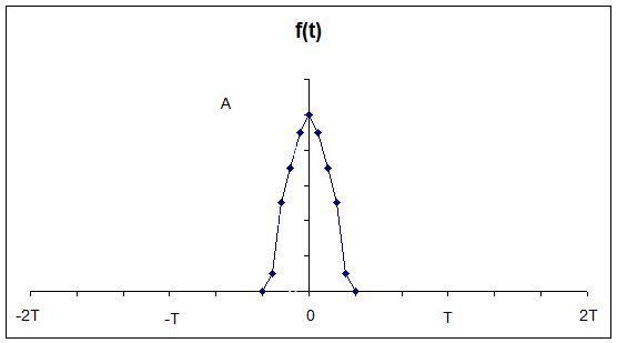
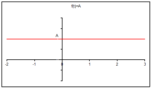
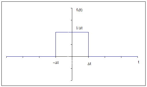
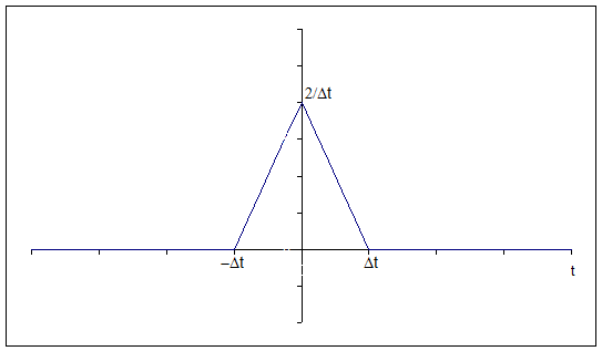
Assume that we have a generalized, time-limited pulse centered at t = 0 as shown below.

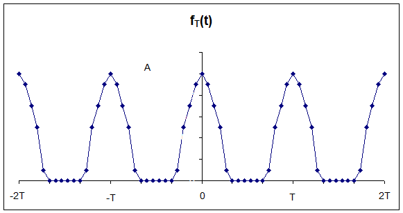
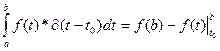
The Fourier Transform of this pulse can be developed by starting with a periodic version of this pulse where the original pulse now repeats every T seconds.

Note:

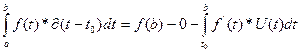
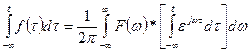
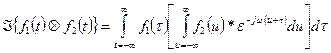
f_T(t) is periodic with period T so we can express it by its exponential Fourier series as

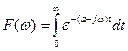
where

and

Now let’s make a small change in notation

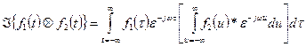
1. w_n = n*w₀

2. F(w_n) = T*F_n

We now have

and

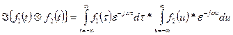
The sum can be rewritten as

or

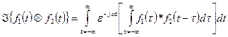
Taking the limit as T ¥

But w₀ = 2p/T so for large T let w₀ Dw and the limit becomes

or since T ¥ implies that Dw 0 and the sum, in the limit, becomes an integral

and

This pair of equations defines the Fourier Transform

1. F(w) is the Fourier Transform of f(t)

2. f(t) is the inverse Fourier Transform of F(w)

3. F(w) is also called the Spectral Density of f(t) as it describes how the energy of the original pulse is distributed as a function of frequency (in radians per second)

I use a backwards upper case script “F” to denote taking the Fourier Transform of a function and the same symbol with a “-1” superscript to denote taking the inverse Fourier Transform.

Example 1

Take the Fourier Transform of the single-sided exponential

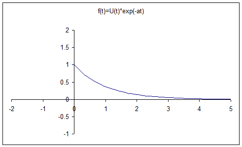
Note that the Fourier Transform is complex. It has a magnitude and a phase. The magnitude is found by multiplying it by its complex conjugate and taking the square root.

This is the magnitude

Now find the phase. First, find the real and imaginary parts.

Therefore the real part is

and the imaginary part is

The phase is then given by

Note: The ArcTan function of your calculator can lie! Its answers always fall between ±90° (±π/2) and the real answer can be in one of the other two quadrants. You should draw a picture to adjust your result as required.
Singularity Functions

We run into special functions when taking the Fourier Transform of functions that have infinite energy. The first of these special functions is the Delta Function

Where G_e(t) is any function from the set of all functions having the properties

1.

2. For all t ¹ 0

Sifting Property of the Delta Function

Integrating the product of the Delta Function with a “well-behaved” function results in “sampling” the “well-behaved” function at the time that the Delta Function goes to infinity. Or

Proof

Use Integration by parts

Let U(t) = f(t) and dV(t) = d(t-t₀)dt

Case 1: a < t₀ < b

Q.E.D

Case 2: t₀ < a or t₀ > b

Q.E.D

Example 2

Take the Fourier Transform of a constant

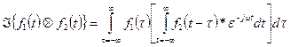
Here the integral can’t be directly computed, we have to approach it as a limiting case. Let’s replace the constant with a parameterized function that equals the constant as its parameter approaches zero, the double-sided exponential function:

Now the Transform becomes:

Let u = -w in the first integral

From our first example this is:

Now we need to take the limit as a 0 to get F(w)

so this is a d-function that goes to ¥ at w = 0 if its integral is a constant.

Let a*x = w

Therefore

Exercises:

1: Find the Fourier Transforms for each of the two pulses

2: Find the transfer function for the simple RC low-pass filter

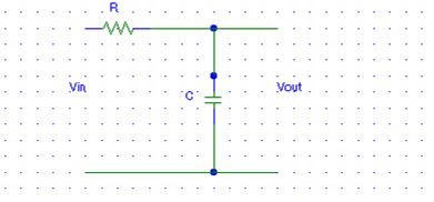
3: Determine the Fourier Transform of the RC low-pass filter output due to each of the pulses in part 1

4: Find the limit of each of the results in part 3 as Dt 0

Properties of the Fourier Transform

Symmetry Property

If f(t) F(w)

Then F(t) 2p f(-w)

Proof:

Therefore

Let u = w and v = t

Now let w = v and t = u

Therefore F(t) 2p f(-w)

And if f(t) is an even function

F(t) 2p f(w)

Linearity Property

If f₁(t) F₁(w)

And f₂(t) F₂(w)

Then [a*f₁(t) + b*f₁(t)] [a*F₁(w) + b*F₂(w)]

Proof:

Results due to the linearity of integration

Scaling Property

If f(t) F(w)

Then for a real

f(a*t)

Proof:

case 1: a > 0 Let x = a*t

or

case 2: a < 0 Again let x = a*t

(Note the limits are now backwards)

or

Therefore including both cases

f(a*t)

Q. E. D.

Note: The compression of a function in the time domain results in an expansion in the frequency domain and vice versa.

Frequency Shifting

If

Then

Proof:

or

Q. E. D.

Note: The Modulation Theorem (very important in communications)

Remember Euler’s Identities

and

therefore

or

similarly

or

Time Shifting

If

Then

Proof:

Q. E. D.

Time Differentiation and Integration

If

Then

And

Proof:

First for differentiation (part 1)

or

Q. E. D. for part 1

Now for integration (part 2)

Interchanging the order of integration

or

Q. E. D. for part 2

Frequency Differentiation

If

Then

Proof:

or

Q. E. D.

The Convolution Theorem

Definition: the convolution of two functions is defined as:

Time Convolution

If

And

Then

Proof:

Therefore

Let u = t - t in the inner integral

Since the inner integral is no longer a function of t, it can be brought out as a constant and this leaves

or

Q. E. D

Frequency Convolution

If

And

Then

Proof: Same method as for time convolution